Lecture 7: A/B Testing and Causality

In this lecture, we discuss A/B testing which is perhaps the most commonly used hypothesis test in industry and scientific research. Similar to what we have seen before, the test compares the null hypothesis to the alternative hypothesis. But the setting of the test is a bit specialized: we have two groups of data samples and we want to test whether the samples from these two groups come from the same distribution. We discuss a specific approach to performing a hypothesis test called permutation testing, which does not require knowing anything about the underlying distribution of the data, though it assumes that the data points are exchangeable under the null distribution (we'll discuss what this means). We then discuss some further implications on causality when we use a specific type of an A/B test called Randomized Controlled Trial.

The Basic Setup in A/B Testing

As mentioned in the lecture summary, A/B tests compare two sets of data samples and their goal is to determine whether the samples came from the same distribution. A/B tests are broadly used in industry (for example, to compare whether the new website design is better than the old one; whether buying an ad generates more traffic; whether offering deals to customers increases the overall profit, etc.) and scientific research (a standard example are randomized control trials where we compare two groups of patients consisting of patients who received a treatment and those who did not). The name A/B testing does not have a special meaning: it comes from naming the two groups of samples by group "A" and group "B."

Notice that this setting is different than the settings we have seen before, because for all previous examples we had some fixed "reference." In particular, in the case of jury panels, we were performing a hypothesis test that tries to determine whether an example (or multiple examples of) jury panel(s) came from the fixed, reference distribution (in the case of jury panels, the reference distribution was the distribution of ethnicities in local population). In A/B testing, there is no fixed reference: we are comparing two random data sets.

To make the discussion of A/B testing more concrete, we will look at a specific example about birth weights of babies born to mothers who were smokers vs non-smokers. This data was collected in a study and is available in 'baby.csv' file that the next cell reads and prints. The example was taken from Section 12.1 in the "Inferential Thinking" book.

A Visual Comparison

To get intuition of the comparison between the two groups, it sometimes helps to visualize it. Looking at the histograms below, the birth weight of babies born to smoking mothers (the "True" histogram on the right) seem shifted to the left compared to the birth weight of babies born to non-smoking mothers. But the plots alone cannot tell us whether this significant, or if any differences are only due to pure chance.

Setting up the Hypothesis Test

As usual, we will set up the hypothesis test by choosing a null hypothesis, an alternative (non-null) hypothesis, a test statistic, and a significance level at which we want to perform the test. In A/B testing, "interesting stuff" happens when the distributions of the two sets of data samples are different. Thus, naturally, our null hypothesis is:

$H_0:$ distributions of birth weights of babies born to smoking and non-smoking mothers are the same.

For the alternative hypothesis, both one-sided hypothesis (that the distribution of birth weight was skewed towards higher values in the group corresponding to babies born to non-smoking mothers) and two-sided hypothesis (that the two distributions are different) make sense. Because A/B tests are commonly performed just to test whether there is an effect or not, we will perform a two-sided test, and so our alternative hypothesis is:

$H_1:$ distributions of birth weights of babies born to smoking and non-smoking mothers are different.

Observe here that there is one random variable (birth weight) per data set that we are using for comparison. If we were comparing it to a reference value (or distribution), we would likely be using the mean birth weight as our test statistic. But here we want to compare the birth weights from two sets of data. Thus it seems like a reasonable choice to consider the difference of means between the two data sets. Observe that under the null hypothesis, this test statistic will have mean zero, but we do not know much more about it.

$S:$ the difference of mean birth weights in group A (babies born to non-smoking mothers) and group B (babies born to smoking mothers).

As usual, we can set our significance level to $\alpha = 0.05$ (statistically significant) or $\alpha = 0.01$ (highly statistically significant). Other values also make sense. For concreteness, let us take $\alpha = 0.05.$
Permutation Test

In the considered example, group A (babies born to non-smoking mothers) has 715 entries, while group B has 459 entries. The observed value of our statistic for this data is 9.266. But is this unusual? That is, can we reject the null hypothesis for this observed value of the statistic? The answer is not clear right away, because we do not know what the distribution of the statistic looks like under the null hypothesis.

A test that is particularly useful in our setting where we do not know the null distribution is called the permutation test. The basic idea is quite simple: if there is no difference between the distributions of groups A and B (i.e., if the null hypothesis holds), then randomly exchanging samples between the groups should not affect the conclusions we make. Note that we are tacitly assuming here that the data satisfies the property called "exchangeability." It means that under the null distribution, the ordering of the data samples has no particular meaning, and so nothing should change if we permute the data samples.

How would this test work? Because we are assuming that permutations have no effect, we would combine all the data in one group, randomly permute the samples, and then assign first 715 samples to group A and the remaining 459 samples to group B. We then compute the test statistic. We do this for all possible permutations and plot the histogram of all the values of the test statistic observed under these permutations. We then look where our initially observed value of the test statistic ($S_{\mathrm{obs}} = 9.266$) falls. If the test statistic falls into a region with less than 5% of data points, we reject the null. Otherwise, we do not reject the null.

You should spot right away that there is a bit of an issue in what I described here. The total number of data samples is 1174. The total number of all possible permutations is thus $1174! \approx 7.28 \cdot 10^{3095}.$ It is impossible to work with this number of permutations! But it is also not necessary. What we are trying to do here is estimate the p-value for our test. P-value is just a probability, a single number. And we have seen many times how to estimate a single number. In particular, we have seen how to compute a confidence interval for the random number of interest. For example, if we use Hoeffding inequality (it applies here, since $p$ can only take values between 0 and 1), we can ensure with 99% confidence that the p-value $\hat{p}$ estimated from $n$ random permutations is from the interval $\hat{p} \in [p - \epsilon, p + \epsilon]$ by ensuring that $n$ and $\epsilon$ are related by

$$ 2 e^{-2n\epsilon^2} \leq 0.01. $$

For example, we could start with $\epsilon = 0.01,$ which would require $n \geq \frac{\log(200)}{2\cdot 0.01^2} \approx 26491.6.$ If we then got $\hat{p} \leq 0.04,$ we could reject the null hypothesis. Or if we had $\hat{p} \geq 0.06,$ we would know that we cannot reject the null. Otherwise, we could perform another test for a smaller $\epsilon,$ and repeat until we can make a conclusive statement.

Causality

A specific type of an A/B test that is heavily used in scientific research is called Randomized Controlled Trial (RCT). The two groups (A and B) in RCTs have the meaning of a "treatment" group and a "control" group. In RCTs, people participating in the trial are randomly assigned to the "treatment" and "control" group, independent of each other. Random assignment is crucial here: it breaks the link between factors other than the treatment that can affect the outcome for the two groups. Thus, it established evidence of causation, meaning that we can claim that any observed effect on the outcome likely came from the treatment.

Beyond the random assignment to the treatment and control group, much of the hypothesis test methodology remains the same. But understanding how randomness enters the picture here is crucial for setting up correct null and alternative hypotheses; for the rest, we can simply use the permutation test as discussed in the previous section.

Potential Outcomes Framework and Controling for Confounding Factors

To understand how causality works, it is necessary to first understand potential outcomes (also called counterfactuals). We'll explain this concept through an example. Suppose that a drug company wants to test a new drug for lower back pain. They recruit people with lower back pain and want to run an A/B test to determine whether the drug is effective.

To perform the test, the drug company assigns each recruited person to one of the two groups: "treatment" and "control." People in the "treatment" group receive the developed drug, while the people in the "control" group receive placebo treatment. After receiving the treatment or the placebo, the recruited patients from both groups are asked whether or not they saw an improvement in low back pain.

For each person, there is an imagined outcome ("pain improved" vs "pain did not improve") based on whether the person was assigned to the treatment group or the control group. This "imagined" outcome is called the "potential outcome" or the "couterfactual." Of course, we only get to observe one value for each person, as each person can only be assigned to one group. So our data would look like this:

Patient # Outcome if assigned to Treatment Group Outcome if assigned to Control Group
1 1 ?
2 0 ?
3 0 ?
4 1 ?
5 ? 0
6 ? 0
7 ? 1
8 ? 0
$\vdots$ $\vdots$ $\vdots$

Now think about the following case. Say we recruited people for our drug experiment from two main places: from UW-Madison and from a retirement home. If we assigned everyone from UW-Madison to the treatment group and everyone from the retirement home to the control group, and more people in the treatment group see improvement in the low back, can we definitively claim that the drug works?

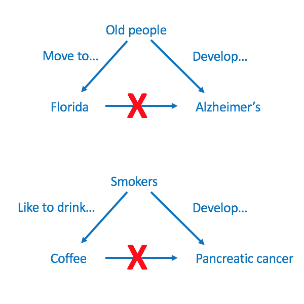
The issue here is that the demographics of the UW-Madison group are likely going to predominantly be young and otherwise healthy people (for example, student athletes who develop back pain from a sports injury or other students who develop back pain due to bad posture while studying). On the other hand, the people from the retirement home are going to be much older and will likely have other health issues. So if the first group has a higher pain improvement rate, that could well be from the fact that they were more likely to recover with no treatment to begin with. These other factors that affect the outcome are called the "confounding factors" (or, colloquially, "confounders"). They prevent us from making inferences about what caused the improvement. Causality is a very important topic, and failing to control for confounding factors can lead to all sorts of wrong conclusions. The following image gives a nice illustration (taken from ACSH based on a Google search)

The first one explains how the association between Florida and Alzheimer's disease does not mean that living in Florida is a risk factor for developing Alzheimer's. It is rather the case that Alzheimer's is primarily diagnosed in advanced age and older people tend to move to Florida. A less obvious example is the association between coffee and pancreatic cancer. There was a study in early 1980s which concluded that coffee caused pancreatic cancer. But the study failed to account for the confounding factor that many people who drank coffee were also smokers. Later studies showed that, in fact, it is smoking that increases the risk of developing pancreatic cancer, whereas coffee itself is not a risk factor.

Controlling for confounding factors can be quite challenging in general, and it is not always possible. Luckily, in the case of Randomized Controlled Trials, there is an easy way to break the link between confounders and the outcomes by assigning participants in the study to the treatment and control group independently (of any other random variables) at random. This way, both the treatment and the control group are equally likely to be affected by any confounding factors. Thus, we can claim that, if there is a difference in the outcomes of the two groups, it can likely be ascribed to treatment.

Setting up a Hypothesis Test

Now that we understand how potential outcomes and confounding work, we understand that the differences in the distribution of the outcomes over the two groups could be ascribed to treatment. Now our A/B test will work similarly as before, and the hypothesis test ingredients are as follows.

$H_0:$ the distributions of the outcomes for the treatment and the control group are the same; any observed differences are purely due to chance.

$H_1:$ the distributions of the outcomes for the treatment and the control group are not the same; the treatment has effect on low back pain.

Test statistic: In the example above, we assigned value 1 for pain improvement and value 0 for no pain improvement. A reasonable test statistic for this case is the difference of mean improvement values between the two groups. We expect that a large absolute value of the test statistic would favor the alternative.

To perform a hypothesis test at a specific significance level (say, $\alpha = 0.05$), similarly as before, we can perform a permutation test to obtain an empirical p-value and reject/not reject the null based on the estimated p-value.

Bibliographical Notes

This lecture is based on Chapter 12 from the "Computational and Inferential Thinking: The Foundations of Data Science" book by Ani Adhikari, John DeNero, David Wagner and on Lecture Notes 21 for 36-705 at CMU (available at https://www.stat.cmu.edu/~larry/=stat705/Lecture21.pdf) by Larry Wasserman.